It's been a while since I've wanted to read Sebastian Raschka's new book, "Build a Large Language Model (from scratch)". Last week, I finally got it and felt the urge to read it with others. So, I tweeted about organizing a study group to go through the book, hoping to get at least four like-minded people interested.

Turns out, over 600 people wanted to join something like that. I quickly put together a Discord server, and people have been joining all week. We're now at almost 700 learners. I named the community AI from Scratch—if this goes well, it would be awesome to continue studying ML/AI methods from scratch together.

Notes (WIP)

I'll add my notes here as I read the book.

Chapter 1: Understanding Large Language Models#

Some years ago, asking a computer to write an email from a list of keywords sounded crazy. This is now a trivial task for an LLM. Earlier NLP models were designed for specific tasks. LLMs perform well across a large variety of tasks.

Large amounts of training data have allowed LLMs to outperform previous approaches.These days, LLMs have around 10-100+ billion parameters (tunable weights). Transformers are the breakthrough that made this possible. They allow models "to pay selective attention to different parts of the inputs when making predictions."

Why Should We Care About Building Custom LLMs?#

• To learn the internal workings of the models. Knowing how the model works also allows us to get better at fine-tuning pre-trained models.
• Privacy concerns.
• To run them on custom devices.
• To decrease latency and reduce API costs.

Stages of Building an LLM:#

1. Collect lots of raw data.
2. Pre-train the model. (Next word prediction).
3. Gather high-quality labeled data for a specific task.
4. Fine-tune the model.

The Transformer Architecture Has Two Modules:#

1. Encoder: Processes input text and encodes it into a series of numerical representations, building embeddings.
2. Decoder: Takes encoded vectors and generates the output text.

Self-Attention Mechanism:#

• Allows the model to weigh the importance of different words or tokens in a sequence relative to each other.
• Enables the model to capture long-range dependencies and contextual relationships.

Model Types:#

• BERT: Focuses on the encoder part of the transformer architecture. It can "see" text in both directions, hence its name, Bidirectional Encoder Representations from Transformers. It was trained using masked word prediction.

• GPT: Focuses on the decoder part, performing next-word prediction, which works well for generative tasks. It’s impressive that it can handle translation tasks, given that it was only trained to predict the next word.

Text completion also works without finetuning:#

• Zero-shot learning: Completes a task without any explicit example.
• Few-shot learning: Completes a task given a few examples of the task.

GPT-Style Models:#

GPT-style models are considered autoregressive models, as they incorporate previous outputs as inputs for future predictions.

Chapter 2: Working with text data#

Preparing input text involves splitting it into individual words and subword tokens, which can then be encoded into vector representations.

Neural networks (NNs) can't process raw text directly. Text data is categorical, which doesn’t align with the mathematical representation that NNs require. To overcome this, we represent words as continuous-valued vectors, known as embeddings.

These embeddings can be created using a neural network layer within the model or by leveraging a pretrained neural network model. There are also embeddings for sentences, paragraphs, and even entire documents—not just for words. In fact, sentence or paragraph embeddings are often used in retrieval-augmented generation (RAG).

RAG combines:

• Text generation
• Retrieval (searching an external knowledge base)

One of the first word embedding models was Word2Vec. It’s a neural network trained to predict either the context of a word given the target word or vice versa. The intuition is that words appearing in similar contexts tend to have similar meanings.

• Higher-dimensional word embeddings capture more nuanced relationships between words.

Today, large language models (LLMs) generate their own embeddings as part of the input layer. These embeddings can be updated during training, allowing them to be fine-tuned for specific tasks.

Tokenizing Text#

• Tokenization involves splitting text into individual tokens.
• During tokenization, we usually avoid making all text lowercase. Capitalization helps LLMs distinguish between proper nouns and common nouns, understand sentence structure, and generate correctly capitalized text.

Converting Text into IDs#

After tokenization, we need to convert tokens into unique IDs for further processing as embedding vectors. This requires creating a vocabulary:

1. Gather all unique tokens in the sample text.
2. Sort them in alphabetical order.
3. Assign a unique ID to each token.

This process enables a mapping from token to ID. Later, we may also need to convert IDs back to tokens, so we should build an inverse dictionary as well.

The SimpleTokenizerV1 class performs tokenization and converts tokens to and from IDs using its encode and decode methods.

class SimpleTokenizerV1:
    def __init__(self, vocab):
        self.str_to_int = vocab
        self.int_to_str = {i:s for s,i in vocab.items()}

    def encode(self, text):
        preprocessed = re.split(r'([,.:;?_!"()\']|--|\s)', text)

        preprocessed = [
            item.strip() for item in preprocessed if item.strip()
        ]
        ids = [self.str_to_int[s] for s in preprocessed]
        return ids

    def decode(self, ids):
        text = " ".join([self.int_to_str[i] for i in ids])

        text = re.sub(r'\s+([,.?!"()\'])', r'\1', text)
        return text

However, this tokenizer has limitations—it can’t handle unknown words (i.e., words not present in the training set).

Adding Special Characters#

To handle unknown words, we can modify our tokenizer to include special tokens such as <|unk|> for unknown tokens and <|endoftext|> to mark the end of a text source.

• When training on batch inputs, we typically use a mask to ignore padding tokens during loss calculation.
• Notably, the GPT model tokenizer doesn’t use the <|unk|> token for out-of-vocabulary words. Instead, it employs Byte Pair Encoding (BPE) to break words into subword units.

Byte Pair Encoding (BPE)#

BPE enables encoding of unknown words without the need for an <|unk|> token. It breaks down text into frequently occurring subword units, allowing words not in the original vocabulary to be represented.

Here’s an example of how BPE works:

Let’s take the sentence: "low low low lower"

1. Initialization: Each unique character is treated as a token. Initially, the sentence appears as:

   ["l", "o", "w", " ", "l", "o", "w", " ", "l", "o", "w", " ", "l", "o", "w", "e", "r"]
   

2. Count Pairs: BPE counts the frequency of adjacent pairs. "lo" and "ow" are frequent pairs. Suppose "lo" is the most frequent.

3. Merge Pairs: The most frequent pair, "lo", is merged into a single token, updating the sentence to:

   ["lo", "w", " ", "lo", "w", " ", "lo", "w", " ", "lo", "w", "e", "r"]
   

4. Repeat the Process: BPE counts pairs again and merges the next most frequent, such as "low", resulting in:

   ["low", " ", "low", " ", "low", " ", "low", "e", "r"]
   

5. Stop Condition: This process continues until a desired vocabulary size or condition is met. Here, BPE stops with the tokens [" ", "low", "e", "r"].

Using BPE, models efficiently encode subword information, handling words absent from the original training data by breaking them into recognizable subwords.

Data Sampling with a Sliding Window#

LLMs are pre-trained by predicting the next word based on previous words. To facilitate this, we create input-target pairs like:

• Input text: ['LLMs', 'learn', 'to', 'predict']
• Target text: ['learn', 'to', 'predict']

Creating Token Embeddings#

The process is as follows:

• Text tokens → Token IDs → Embedding vectors

Embedding vectors are typically initialized with random values, which are optimized during training.

Encoding Word Positions#

Word embeddings, as described, don’t capture the position of words in a sentence. For example, a Token ID:7 maps to the same embedding vector regardless of its place in a sentence. This consistency is good for reproducibility, but since self-attention is also position-agnostic, we need a way to encode positional information in the model.

Two options are commonly used:

1. Absolute Positional Embeddings: Assigns a unique embedding for each position within the input sentence.

   • Example:
     • Token embedding: [1, 1, 1]
     • Positional embedding: [1.1, 1.2, 1.3]
     • Final embedding = Token embedding + Positional embedding = [2.1, 2.2, 2.3]

2. Relative Positional Embeddings: Focuses on the relative distances between tokens rather than their exact positions. This approach helps generalize better to sequences of varying lengths.

OpenAI’s GPT models use absolute positional embeddings, which are optimized during training rather than fixed or predefined.

Chapter 3: Coding attention mechanisms#

This chapter builds the multi-head attention mechanishm from the ground up by starting from a simple version to multi-head attention.

1. Simple self-attention (no trainable weights): Introduces the general idea
2. Self-attention with trainable weights: Uses trainable weights that form the basis of the mechanism
3. Causal attention: Allows a model to consider only previous and current inputs, ensuring temporal order during text generation
4. Multi-head attention: Combines self-attention and causal attention to enable the model to simultaneously use information from different representation subspaces

The Problem with Modeling Long Sequences#

Before LLM architectures (without self-attention):

• Word-by-word translation didn't work as it ignores grammatical structures of both source and target languages
• Generated translations require access to words that appear earlier or later in the original sentence
• Encoder-decoder architectures were commonly used to tackle this issue
• RNNs were the most popular encoder-decoder architecture for translation

In the encoder-decoder approach:

• Encoder reads the entire text first and updates its hidden state at each step
• Decoder takes the hidden state, generates the translated sentence, and updates the hidden state to carry the context
• The hidden state acts as an embedding vector

Limitations of encoder-decoder RNNs:

• RNNs can't access earlier hidden states from the encoder during the decoder phase
• They rely only on the current hidden state
• This results in loss of context, which motivated the design of attention mechanisms

Capturing Data Dependencies with Attention Mechanisms#

• The popular self-attention mechanism was inspired by the Bahdanau attention mechanism
• Bahdanau attention modifies an RNN encoder-decoder so the decoder can access different parts of the input sequence at each decoding step
• Self-attention allows each position in the input sequence to consider the relevancy of all other positions when computing the representation of a sequence

Attending to Different Parts of the Input with Self-Attention#

The "self" in self-attention relates to the mechanism's ability to compute attention weights relating different positions within a single input sequence.

Simple Self-attention (no trainable weights)#

Goal: Compute the context vector $Z^{(i)}$ for each input element $X^{(i)}$

Ingredients:

• Token embeddings for each token $X^{(i)}$
• Embedded token query. Each token will play the role of token query. In the next example $X^{(2)}$ will be the token query.

Process:

1. Start with token embeddings for each token
2. Pick a token query. e.g.; $X^{(2)}$
3. Compute the dot product between the query token, $X^{(2)}$, and all the other token embeddings. The result from each of this dots produts is called the attention score ($\omega$). e.g.; $\omega_{21} = X^{(2)} \cdot X^{(1)}$ Higher dot product indicates higher similarity and attention score.
4. Next, normalize the attention scores to obtain attention weights $\alpha$. We can do this by applying softmax.
5. The last step is to compute the context vector $Z^{(i)}$. For $Z^{(2)}$ we perform a weighted sum of all the input vectors $X^{(1)}$ to $X^{(T)}$ by their the attention weights $\alpha_{21}$ to $\alpha_{22}$ . Context vectors create enriched representations by adding information from all other input elements

Flow: $X$ (input token embeddings) → ω (attention scores) → α (normalized attention weights) → Z (context vector)

Self-attention with Trainable Weights#

Also called scaled-dot product attention, this version adds trainable matrices that are updated during model training to create better context vectors.

Computing Attention Weights Step by Step#

Three trainable matrices:

• $W_q$ : Query matrix
• $W_k$ : Key matrix
• $W_v$ : Value matrix

Process:

1. Project embedded input tokens into query ($q$), key ($k$), value ($v$) vectors
   1. $q^{(i)}$ = $X^{(i)}$ $W_q$
   2. $k^{(i)}$ = $X^{(i)}$ $W_k$
   3. $v^{(i)}$ = $X^{(i)}$ $W_v$
2. Get the attention scores by computing the the dot product between $q$ and $k$. e.j.; $\omega_{21} = q^{(2)} \cdot k^{(1)}$
3. Scale attention scores by dividing by the square root of the embedding dimension of keys
4. Apply softmax to get attention weights $\alpha$
5. Multiply each value vector $v$ with respective attention weights $\alpha$ and sum to get context vectors $Z$

Causal Attention#

Causal attention restricts a model to only consider previous and current inputs in a sequence when processing any given token while computing attention scores.

Standard self-attention allows access to the entire sequence at once. Causal attention is also called masked attention.

In causal attention, we mask out the attention above the diagonal and normalize the non-masked attention weights such that the attention weights sum up to 1 in each row.

Masking Attention Weights with Dropout#

When applying dropout to an attention weight matrix with a rate of 50%, half of the elements in the matrix are randomly set to zero. To compensate for the reduction, the remaining elements of the matrix are scaled up by a factor of 1/0.5 = 2. This is done to maintain the balance of the attention weights, ensuring that the average influence of the attention mechanism remains consistent during training and inference.

Multi-head Attention#

Multi-head attention divides the attention mechanism into multiple "heads," each operating independently. The idea of multi-head attention is to run the attention mechanism multiple times in parallel with different learned linear projections.

Chapter 4: Implementing a GPT Model from Scratch to Generate Text#

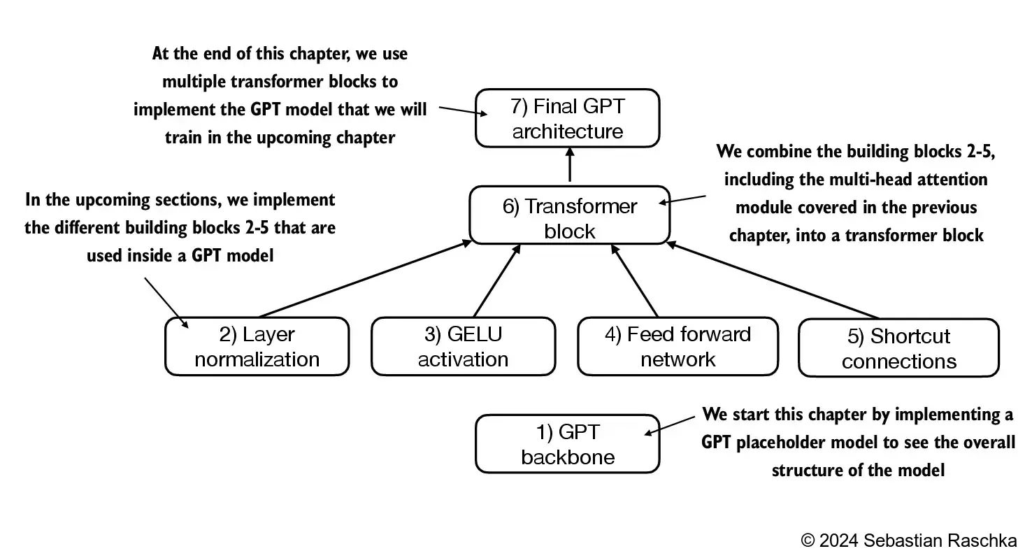
Sebastian takes a step by step approach for teaching how to code the general LLM architecture. We start by coding a GPE backbone, with some place holder methods and gradually improve on it untill we have the general implementation.

Steps for Implementation:#

1. GPT Backbone
2. Layer Normalization
3. GELU Activation
4. Feed Forward Network
5. Shortcut Connections
6. Transformer Block
7. Final GPT Architecture

Normalizing Activations with Layer Normalization#

Layer normalization addresses this by improving the stability and efficiency of neural network training.

Key Idea:#

Adjust the outputs of a neural network layer to have a mean of 0 and a variance of 1, which speeds up convergence.

This is typically done:

• Before and after the multi-head attention module.
• After the final output layer.

Implementing a Feed Forward Network with GELU Activations#

GELU: Gaussian Error Linear Unit

This activation function offers improved performance for deep learning models. In GPT-3, an approximation of GELU was used, derived through curve fitting.

Insert GELU Formula Here

GELU provides small, non-zero outputs for negative values. This allows neurons with negative inputs to still contribute to learning, albeit to a lesser extent than positive inputs.

Adding Shortcut Connections#

Vanishing Gradient Problem:#

Gradients, which guide weight updates during training, become progressively smaller as they propagate backward through the layers. This makes it difficult to effectively train earlier layers.

Solution:#

A shortcut connection creates an alternative, shorter path for the gradient to flow through the network, bypassing one or more layers.

Connecting Attention and Linear Layers in a Transformer Block#

A transformer block combines the causal multi-head attention module (discussed in the previous chapter) with linear layers and the feed-forward neural network implemented earlier. Additionally, it employs dropout and shortcut connections.

Inputs and Outputs of a Tranformer blog share the same shape#

The preservation of shape throughout the transformer block architecture is not incidental—it is a crucial design aspect. This allows the block to be applied effectively to sequence-to-sequence tasks, where each output vector directly corresponds to an input vector, maintaining a one-to-one relationship.

Chapter 5: Pretraining on Unlabeled Data#

Work in progress...